Mnist digit classification with Tensorflow on Android

Emmanuele Villa

Emmanuele Villa

How to train a neural network online and import the trained model in android

I’ve started to experiment with tensorflow after a very deep course, and -since I’m mainly a mobile developer- of course I wanted to try to use a neural network inside an app!

Before that, if you are italian and interested in tensorflow, I’m recording a course on youtube

Now, without further ado, lets go through the process step by step!

Step 1: Create, train and export the model

For this step I’ve used google colab, and you can find the full colab file along with the app code in the github repository linked at the end.

Step 1a: Import the modules

Since the module we need is not already installed in the google colab runtime, we need to install it with:

				
					!pip install tflite-support


Be aware that after the install is complete, you may need to restart the runtime and execute the cell again!

After this step we can import all the modules we’ll need later:

				
					import tensorflow as tf
import pandas as pd
import matplotlib.pyplot as plt
import numpy as np
from tflite_support import flatbuffers
from tflite_support import metadata as _metadata
from tflite_support import metadata_schema_py_generated as _metadata_fb
import os, random
				
			
Step 1b: Prepare the dataset

Before training the model we of course need to import the mnist dataset and split it in train, test and validation.

After the download, we need to expand the image dimensions to fit what the convolutional layer is expecting.

We also need to create a labels.txt file that we’ll use to export the model to tensorflow lite:

				
					mnist = tf.keras.datasets.mnist
(train_data, train_labels), (test_data, test_labels) = mnist.load_data()
val_data = test_data[:5000]
val_labels = test_labels[:5000]

train_data = tf.expand_dims(train_data, -1)
test_data = tf.expand_dims(test_data, -1)
val_data = tf.expand_dims(val_data, -1)

!echo "0\n1\n2\n3\n4\n5\n6\n7\n8\n9" > labels.txt


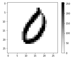
After correctly visualizing the data using matplotlib we are ready to create our neural network model!

Step 1c: Create the model
Before creating the model, a little excursus regarding the layers that we’ll be using:
The convolutional layer contains N filters of MxM size, takes an image as input and outputs N images, each one created by applying the Nth filter to the Nth image, in this way:
 
 
The MaxPooling layer contains a MxM shape, takes N images as input and outputs N images. Same as before, the Nth output image is created by applying the MxM shape to the input image, in this way:
 
These two layers are quite always used together: the first one is used to highlight the features of the image and the second to reduce the image size, which also results in highlighting features because it takes the maximum or the average value of the pixels.
 
I made a video (in italian) about this operation that you can find at this url. 
 
Our network will expect a 28×28 image with values ranging from 0 to 255: for this reason in the first layer we apply a lambda layer that normalize the values in the (0,1) range.
After that, there’ll be a convolutional layer with 32 5×5 filters, a max pooling 2d layer and then another conv+maxpooling pair, this time with 16 5×5 filters.
After that, we have a flatten filter, a dense filter with 64 neurons and the last one with 10 neurons, the same number as our labels. This last time the activation function is softmax, since we want the outputs to be in a probability form
 
				
					model = tf.keras.models.Sequential(
    [
        tf.keras.layers.Lambda(lambda x : tf.cast(x, tf.float32) / 255.0),
        tf.keras.layers.Conv2D(32, 5, activation="relu"),
        tf.keras.layers.MaxPooling2D(),
        tf.keras.layers.Conv2D(16, 5, activation="relu"),
        tf.keras.layers.MaxPooling2D(),
        tf.keras.layers.Flatten(),
        tf.keras.layers.Dense(64, activation="relu"),
        tf.keras.layers.Dense(10, activation="softmax")
    ]
)


Now we need to compile the model (which means to pass the loss, optimizer and metrics values) and fit it using the train data:

				
					model.compile(
    loss=tf.keras.losses.SparseCategoricalCrossentropy(),
    optimizer=tf.keras.optimizers.SGD(),
    metrics=["accuracy"]
)

history = model.fit(train_data, train_labels, epochs=15, validation_data=(val_data, val_labels))


After 15 epochs, our model reached 99% accuracy on the train data, 98.28% on the validation data and 98.89% on the test data!

We are now ready to export it in the tensorflow lite format, which is as simple as:

				
					# Convert the model to tf lite
converter = tf.lite.TFLiteConverter.from_keras_model(model)
tflite_model = converter.convert()

# Save the model to file
with open('model.tflite', 'wb') as f:
  f.write(tflite_model)


Of course, this seem maybe a lit too easy because we are working with a very small model: with very complicated neural networks you may incur in errors when exporting it to the tensorflow lite format, since -as the name suggests- it doesn’t support everything that tensorflow core does.

To smoothen the model usage in the android app, we also need to add some long and annoying metadata regarding input, outputs, labels and stuff. This is just a very long boilerplate so I won’t burden this post with it. You can find it in the full colab file I saved on github, along with the last step: downloading the model.tflite file

				
					from google.colab import files
files.download("model.tflite")


Step 2: Create a paint app with compose

We want to be able to draw and query the model about the digit, so we need to build a small UI that let us do that.

I’m not a fan of developing UI stuff, so I managed to find this very cool sample app that handles it beautifully with the jetpack compose library from which I took inspiration (and code) to develop this:

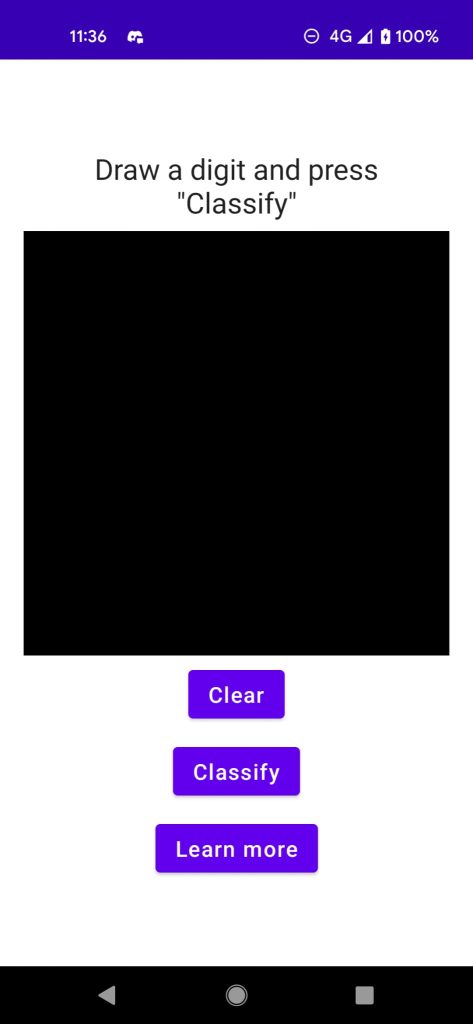
Very simple: draw in the black box, press “Clear” to delete, “Classify” to query the model and “Lear more” to land on this page. Good! We are now ready to prepare the input data

Step 3: Convert the Canvas to a Tensor

The first step to prepare the input data is converting the draw that we have, in the form of a Canvas, to a Bitmap image.

I did this using this awesome CaptureBitmap Composable that convert any composable to an image, with some kind of dark magic I haven’t investigated.

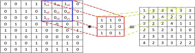
But this conversion is not enough! The Tensorflow Lite Android wrapper generator seems broken at the moment and I wasn’t able to generate a wrapper that handles the bitmap conversion to a tensor, so I’ve converted it myself.

The model expect a bytebuffer object composed by 784 bytes (1x28x28x1), but after resizing our bitmap’s buffer contains 4 times that: 3136 bytes total for the argb channel.

So, we’ll create a custom buffer by reading the red value, since the rgb values are all the same in our greyscaled image:


					fun getGrayscaleBuffer(bitmap: Bitmap): ByteBuffer {
    // allocate custom buffer
    val mImgData: ByteBuffer = ByteBuffer
        .allocateDirect(28 * 28)
    mImgData.order(ByteOrder.nativeOrder())
    
    // get all pixels
    val pixels = IntArray(28 * 28)
    bitmap.getPixels(pixels, 0, width, 0, 0, width, height)
    for (pixel in pixels) {
        // transform the color to byte
        val color = Color.red(pixel)
        val byte = color.toByte()
        // and add it to the buffer
        mImgData.put(byte)
    }
    return mImgData
}

// Take the composable snapshot
val bitmap = snapShot.invoke()

// Scale to 28x28
val scaled = Bitmap.createScaledBitmap(bitmap, 28, 28, false)

// Create a 1x28x28x1 tensor buffer
val image = TensorBuffer.createFixedSize(
    intArrayOf(1, 28, 28, 1), DataType.UINT8)

// Load the grayscale image into the buffer
image.loadBuffer(getGrayscaleBuffer(scaled))


Step 4: Query the model

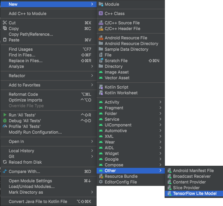
Before we can query the model, we can finally import the tflite file into our android project. This is done by simply right click on the module folder and select the tf lite format. This will also automagically add all the needed dependencies in the gradle file!

Now, we can query it like so:

				
					val image = TensorBuffer.createFixedSize(
intArrayOf(1, 28, 28, 1), DataType.UINT8)

image.loadBuffer(getGrayscaleBuffer(scaled))

// pass the byte buffer to the model
val outputs = model.process(image)

// read the list of probabilities
val probability = outputs.probabilityAsCategoryList

// convert it to int because I like it
val intProb = probability.map { (it.score * 100).toInt() }

// find the max value
val maxProb = intProb.maxOrNull() ?: 0

// find the index of the max value, which coincides with our label
val index = intProb.indexOf(maxProb).toString()

// close the model at the end of the operations
model.close()


We got it! We have a prediction! We can now print it in a flawless way:

				
					Toast.makeText(
                context,
                "Predicted $index with $maxProb% probability",
                Toast.LENGTH_SHORT
            ).show()


I hope this was as interesting to read as it was interesting to experiment on!

What you can do now?

  1. See the app in action on youtube!
  2. Download the app from the play store
  3. Have a look at the colab and app code on github
  4. Leave a heart here, a star on github and let me know what you think in the comments!

Share:

Facebook
Twitter
Pinterest
LinkedIn

Leave a Reply

Your email address will not be published. Required fields are marked *

On Key

Related Posts